Asset Pricing: Martingales and the Markov Property

Below I discuss a curious feature that arises from the Markov property in an asset pricing model.

Asset returns $R_{t}$ are functionals of a Markov chain $R_{t+1} = r \cdot X_{t+1}$ where $r \in \mathbb{R}^{S}$ , $x_{t} \in X \,$ and $\mathbb{N} \ni S:=\#X < \infty$ . Dynamics are governed by the Markov transition kernel $\mathcal{M}$ , which contains the conditional transition probabilities $\mathcal{M}_{i,j} := Pr\left(X_{t+1} = x_{t+1,j}|x_{t,i}\right)$ for ordered pairs $(x^{[i]}, x^{[j]}) \in X \times X$ .

Realizations are normalized to be indicator functions $x_{t,j} \in \{0,1\}$ . The state of the system is characterized by the indicator vector $1(x_{t}) \in \mathbb{R}^{S}$ , where the column of indicators is zero everywhere other than the realized coordinate.

Expected returns are $\mathbb{E}[R_{t+1}|x_{t}] = r \cdot \mathcal{M}'1(x_{t})$ . Under the Markov transition decomposition $\mathcal{M}' = \mu_{0} \iota' + \mathcal{M}_{\boldsymbol{\gamma}}'$ with $\iota:=1_{S \times 1}$ and leading eigenvector $\mu_{0}' = \mu_{0}' \mathcal{M}$ , expected returns can be written $\mathbb{E}[R_{t+1}|x_{t}] = r \cdot \mu_{0} + r \cdot \mathcal{M}_{\gamma}' 1(x_{t})$ .

The rows of the transition matrix sum to one. Preservation of probability enforces a zero-sum condition $\mathcal{M}_{\boldsymbol{\gamma}} \iota = 0_{S \times 1}$ . Assuming in addition that $\text{rank}\left(\mathcal{M}\right) > 1$ , the rows of $\mathcal{M}_{\boldsymbol{\gamma}}$ contain both positive and negative values.

The rows of $\mathcal{M}_{\gamma}$ describe the local redistribution of probabilities away from their invariant values. Because they contain negative entries in every nontrivial case, they are generalized probabilities.

The following simulations illustrate the phenomena of probability redistribution and dimension reduction for a Markov chain.

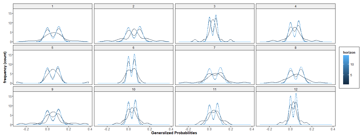
Each enumerated facet corresponds to a state of a 12-state Markov process. Integer powers of a Markov transition matrix capture transition probabilities over integer horizons. The plots show smoothed frequency counts of generalized probability values for successive horizons (black lines are early iterations – blue lines are later). The top panel shows distributions of probabilities relevant for forecasting k as k goes from periods 1-15, the lower shows horizons from 1 to 8.

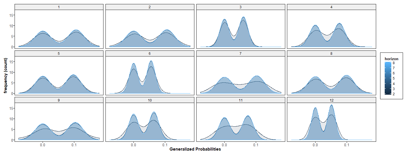
The probability of each state is approximately bimodal for mid-range forecasts. For limiting long-run forecasts, the distributions are degenerate with all mass assigned to nonzero probabilities at the invariant values, represented by the right modes. Probability re-distributional effects are represented by the left modes.

An initial transition matrix, say $\mathcal{M}$ , contains probabilities for each state in terms of the conditional probabilities of arriving in that state from each of every other state; it also contains the probability of staying in that state. The collection of these numbers is the initial distribution of probabilities for each state. This probability becomes less dependent on conditioning as the forecasting horizon grows, ultimately approaching its invariant or long-run value (right modes). The corresponding conditional probability re-distributions approach zero, but are non-negligible for finite-horizon forecasts (left modes).

In any finite sample, ergodic time series are generated by transition probabilities with some conditional dependence. Think, say, of the curve corresponding to the horizon h=8, and consider repetitions of a transition with the corresponding probabilities. This new process is also a Markov process, with an approximate 2-factor structure for dynamics. The trailing factor drives fluctuations that die out in large-time forecasts but are predictable in finite samples.